heritable - Flexible heritability estimation from complex linear mixed models

AAGIverse Community Event

Yidi Deng, Fonti Kar, Patrick Li, Emi Tanaka

Research School of Finance, Actuarial Studies and Statistics, ANU

16th July 2026

Project overview

Given genotypes and their observed traits in a trial, heritability helps breeders decide whether the trial contains enough genetic signal for selection.

This project aims to make heritability estimation from LMMs more accessible, flexible, and interpretable.

It brings together:

• 6 commonly used heritability estimators (Paul Schmidt et al. 2019)
• confidence interval based on parametric bootstrap
• support for different model object (asreml and lme4), with flexible model constructs
• G×E extensions for environment-specific and environment-averaged heritability
• a companion paper on estimator relationships and statistical properties

Acknowledgement

Dr. Fonti Kar made the foundational contribution to this project.

Software availability

Thanks to Fonti’s earlier work, heritable is already available on CRAN.

The CRAN version only supports broad-sense heritability estimation on relatively simple model.

# # Install the CRAN version
# install.packages("heritable")

fit <- lme4::lmer(y ~ rep + (1|gen), data = heritable::lettuce_phenotypes)

heritable::H2(fit, target = "gen")

   Cullis     Oakey    Piepho     Delta  Standard 
0.7737597 0.7737597 0.7725430 0.7737597 0.7725517 

The current development version is maintained on GitHub, mainly on the narrow-sense branch (https://github.com/anu-aagi/heritable/tree/narrow-sense).

Manuscript in preparation

Beyond implementing existing estimators

We re-derive different heritability estimators within a unified mathematical framework that:

• connects different estimators

• provides a comprehensive understanding of their underlying estimands

• extends heritability definitions to more flexible model settings

Extensive numerical studies show that heritability estimation is strongly design-dependent.

Heritability as variance partitioning

Heritability estimation is fundamentally about partitioning variation under a LMM.

\mathbf{y} = \mathbf{X}\boldsymbol{\beta} + \mathbf{Z}_g\mathbf{u}_g + \mathbf{Z}_{ge}\mathbf{u}_{ge} + \boldsymbol{\varepsilon}

where

\mathbf{u}_g \sim N(\mathbf{0}, \mathbf{G}_g), \qquad \mathbf{u}_{ge} \sim N(\mathbf{0}, \mathbf{G}_{ge}), \qquad \boldsymbol{\varepsilon} \sim N(\mathbf{0}, \mathbf{R})

This model gives arise to three related variance quantities:

• Phenotypic variance: V_P = \mathrm{Var}(\mathbf{d}^\top \mathbf{y})

• Genetic variance: V_G = \mathrm{Var}(\mathbf{c}^\top \mathbf{u}_g)

• Prediction error variance: V_{\mathrm{PEV}} =\mathrm{Var}\left[\mathbf{c}^\top\left(\mathbf{u}_g - \hat{\mathbf{u}}_g\right)\right], \hat{\mathbf{u}}_g is the BLUP of \mathbf{u}_g

Two classes of heritability estimators

Two classes of estimators emerge from decomposing two different notions of variance:

Phenotypic variance partition

V_P = \mathrm{Var}(\mathbf{d}^\top \mathbf{y}) = \underbrace{\mathrm{Var}(\mathbf{d}^\top \mathbf{Z}_g\mathbf{u}_g)}_{V_G} + \mathrm{Var}(\mathbf{d}^\top \mathbf{Z}_{ge} \mathbf{u}_{ge}) + \mathrm{Var}(\mathbf{d}^\top \mathbf{\epsilon}) H^2 = V_G/V_P

Genetic variance partition

V_G = \mathrm{Var}(\mathbf{c}^\top \mathbf{u}_g) =\mathrm{Var}(\mathbf{c}^\top \hat{\mathbf{u}}_g) + \underbrace{\mathrm{Var}\left[\mathbf{c}^\top\left(\mathbf{u}_g - \hat{\mathbf{u}}_g\right)\right]}_{V_{\text{PEV}}} H^2 = 1 - V_{\text{PEV}}/V_G

Phenotypic variance partition

This class includes the Standard, Delta (BLUE), and Piepho estimators. Different estimator differs by how the linear functionals are defined:

• Standard (Falconer 1996): \mathbf{d}_{ij} is defined for a genotype pair (i, j) such that \mathbf{d}_{ij}^\top \mathbf{y} represents the phenotypic mean difference between genotypes i and j: \mathbf{d}_{ij}^\top \mathbf{y} = \bar{y}_i - \bar{y}_j.

• Delta (BLUE) (P. Schmidt et al. 2019): same pairwise idea, but \mathbf{d}_{ij} maps \mathbf{y} to BLUE contrasts from a counterpart model where genetic effects are fitted as fixed: \mathbf{d}_{ij}^\top \mathbf{y} = \hat{\beta}_{g_i} - \hat{\beta}_{g_j}.

• Piepho (Piepho and Mohring 2007): aggregated \Delta^{\text{BLUE}} heritability for isotropic \mathbf{G}_g

Genetic variance partition

Similarly, the Delta (BLUP), Cullis, and Oakey estimators differ in how they define linear functionals of genetic effects.

• Delta (BLUP) (P. Schmidt et al. 2019): \mathbf{c}_{ij} is defined for genotype pair (i, j) for genetic effect contrast: \mathbf{c}_{ij}^\top\mathbf{u}_g = u_{g_i} - u_{g_j}

• Cullis (Cullis, Smith, and Coombes 2006): aggregated \Delta^{\text{BLUP}} heritability for isotropic \mathbf{G}_g

• Oakey (Oakey et al. 2006): \mathbf{c} is defined in a model dependent way to maximize heritability: \arg\max_\mathbf{c} 1- \frac{\mathrm{Var}\left[\mathbf{c}^\top\left(\mathbf{u}_g - \hat{\mathbf{u}}_g\right)\right]}{\mathrm{Var}(\mathbf{c}^\top \mathbf{u}_g)}

Back to the original formulation

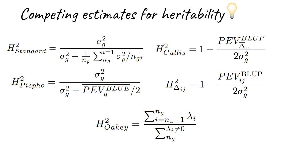
A slide from Fonti’s talk

We can define our own linear functionals

The calculation follows the same principle as long as the genetic effect of interest can be isolated as a random effect component.

\mathbf{y} = \mathbf{X}\boldsymbol{\beta} + \color{red}{\mathbf{Z}_g\mathbf{u}_g} \color{black} + \mathbf{Z}_{ge}\mathbf{u}_{ge} + \boldsymbol{\varepsilon}

Extension to G×E is straightforward

G×E effects can be incorporated into the heritability definition by defining and decomposing variance of the full random effect vector \mathbf{u} = \begin{bmatrix} \mathbf{u}_g \\ \mathbf{u}_{ge} \end{bmatrix}, Let \tilde{\mathbf{c}} be a linear functional defined on \mathbf{u}, then H^2_{\text{GVP}} = 1 - \frac{V_{\text{PEV}}}{V_G} = 1- \frac{\mathrm{Var}\left[\tilde{\mathbf{c}}^\top\left(\mathbf{u} - \hat{\mathbf{u}}\right)\right]}{\mathrm{Var}(\tilde{\mathbf{c}}^\top \mathbf{u})}.

This extension can be applied also to phenotypic variance partitioning.

Stratified and marginal heritability

Stratified heritability

We can define stratified heritability with a functional \tilde{\mathbf{c}}_{ijk} that contrasts genetic effects within an environment k, such that \tilde{\mathbf{c}}_{ijk}^\top\mathbf{u} = u_{g_i} + u_{ge_{ik}} - (u_{g_j} + u_{ge_{jk}})

Marginal heritability

We can also define marginal heritability by \tilde{\mathbf{c}}_{ij} that contrasts genetic effects averaged across environments, such that \tilde{\mathbf{c}}_{ij}^\top\mathbf{u} = \left( u_{g_i} + \sum_k \mathbb{E}[z_{ge_{ik}}] u_{ge_{ik}} \right) - \left(u_{g_j} + \sum_k \mathbb{E}[z_{ge_{jk}}] u_{ge_{jk}} \right)

Usage

There are three important arguments for the key functions H2 and h2:

• target: specifying the model component on which heritability is estimated

• marginal: whether to compute marginal heritability

• stratification: specifying the environmental strata at which heritability is estimated

We use a lettuce breeding dataset for resistance to downy mildew for demonstration (Hadasch et al. 2016)

# gen: genotype
# loc: location
# rep: replicates
# Fit a asreml model
model <- asreml::asreml(
  fixed = y ~ rep,
  random = ~ gen + loc + gen:loc,
  trace = FALSE, data = heritable::lettuce_phenotypes)

Online License checked out Thu Jul 16 21:54:48 2026

Board-sense heritability

Main heritability

heritable::H2(model, target = "gen", marginal = FALSE)

   Cullis     Oakey    Piepho     Delta  Standard 
0.7818483 0.7818483 0.7806164 0.7818483 0.7750432 

Marginal heritability

heritable::H2(model, target = "gen", marginal = TRUE)

   Cullis     Oakey    Piepho     Delta  Standard 
0.8918403 0.8816483 0.8895923 0.8918403 0.8895923 

Stratified heritability at location L1

heritable::H2(model, target = "gen", stratification = data.frame(loc = "L1"))

   Cullis     Oakey    Piepho     Delta  Standard 
0.7870171 0.7780585 0.7250283 0.7870171 0.7250283 

Narrow-sense heritability

Same usage, differs in the modelling stage

We model known additive genetic variance structure using the vm special in asreml:

# lettuce_GRM: genomic relationship matrix defining the known variance structure
# Fit a asreml model
model <- asreml::asreml(
  fixed = y ~ rep,
  random = ~ vm(gen, source = heritable::lettuce_GRM)*idv(loc),
  trace = FALSE, data = heritable::lettuce_phenotypes)

An additional argument source is required by h2:

heritable::h2(model, target = "gen", marginal = FALSE,
              source = list(`heritable::lettuce_GRM` = heritable::lettuce_GRM))

   Cullis     Oakey    Piepho     Delta  Standard 
0.8757316 0.6572500 0.8528437 0.8748936 0.8468753 

Confidence Interval

To compute CI, simply run confint on saved heritable objects

# Store the `heritable` object
my_h2 <- heritable::h2(model, target = "gen", marginal = FALSE,
              source = list(`heritable::lettuce_GRM` = heritable::lettuce_GRM))

# Run confint generic!
confint(my_h2, parallel = "snow", ncpus = 3)

             2.5 %    97.5 %
Cullis   0.8323671 0.9374830
Oakey    0.5911317 0.7334316
Piepho   0.8028306 0.9190309
Delta    0.8283260 0.9346294
Standard 0.7888382 0.9111070

The function supports parallel computing to accelerate parametric bootstrap.

Works for complex models

Deep nesting

lme4::lmer(
  y ~ Type * Treatment * Stage +
    (1 | Genotype) + (Stage | Genotype / Treatment) +
    (1 | Date) + (1 | Plot / Replicate),
  data = df
) |>
  heritable::H2(target = "genotype")

   Cullis     Oakey    Piepho     Delta  Standard 
0.5793787 0.5969357 0.4619369 0.5793787 0.4592437 

Residual modeling

asreml(
  fixed = y ~ 1,
  random = ~ Line + Range + Row + RowRep:ColRep,
  residual = ar1(Range):ar1(Row),
  data = df
) |>
  heritable::H2(target = "Line")

   Cullis     Oakey    Piepho     Delta  Standard 
0.9545024 0.9545024 0.9544771 0.9545024 0.9518358 

Future development

More variance structures

heritable needs to parse asreml variance modeling specials and convert variance estimates into variance matrices.

• Some structures are already supported

• More structures can be added

Custom heritability definitions

Future versions could allow users to provide their own linear functionals, such as \mathbf{d} or \mathbf{c}.

This would support custom heritability definitions for user-defined contrasts.

More model objects

Patrick is working on glmmTMB

Reference

Cullis, Brian R, Alison B Smith, and Neil E Coombes. 2006. “On the Design of Early Generation Variety Trials with Correlated Data.” Journal of Agricultural, Biological, and Environmental Statistics 11 (4): 381–93.

Falconer, Douglas Scott. 1996. Introduction to Quantitative Genetics. Pearson Education India.

Hadasch, Steffen, Ivan Simko, Ryan J Hayes, Joseph O Ogutu, and Hans-Peter Piepho. 2016. “Comparing the Predictive Abilities of Phenotypic and Marker-Assisted Selection Methods in a Biparental Lettuce Population.” The Plant Genome 9 (1): plantgenome2015–03.

Oakey, Helena, Arūnas Verbyla, Wayne Pitchford, Brian Cullis, and Haydn Kuchel. 2006. “Joint Modeling of Additive and Non-Additive Genetic Line Effects in Single Field Trials.” Theoretical and Applied Genetics 113 (5): 809–19.

Piepho, Hans-Peter, and Jens Mohring. 2007. “Computing Heritability and Selection Response from Unbalanced Plant Breeding Trials.” Genetics 177 (3): 1881–88.

Schmidt, Paul, Jens Hartung, Jörn Bennewitz, and Hans-Peter Piepho. 2019. “Heritability in Plant Breeding on a Genotype-Difference Basis.” Genetics 212 (4): 991–1008. https://doi.org/10.1534/genetics.119.302134.

Schmidt, P, J Hartung, J Rath, and H-P Piepho. 2019. “Estimating Broad-Sense Heritability with Unbalanced Data from Agricultural Cultivar Trials.” Crop Science 59 (2): 525–36.